QGIS for Drone Data: The Complete Workflow Guide

You’ve processed your drone data. The orthomosaic is a 2 GB GeoTIFF sitting on your desktop. The DEM is ready. Maybe you’ve got a point cloud too. Now what?

If you’re not paying for ArcGIS Pro — or you just don’t want to — QGIS is the answer. Free, open-source, and as of version 3.44 LTR, genuinely capable of handling everything from orthomosaic display to contour generation to point cloud visualization. No license fees. No subscription. No vendor lock-in.

The problem is that most QGIS-for-drone-data content is either documentation written for GIS academics or five-minute YouTube walkthroughs that skip every detail that matters. This guide covers the complete practitioner workflow — from importing your first orthomosaic to sharing deliverables on a tablet in the field.

A westman, via Wikimedia Commons, CC0 1.0

What You Need: QGIS 3.44 LTR

As of spring 2026, QGIS 3.44 ‘Solothurn’ is the current Long Term Release. Download it from qgis.org/download. The LTR is what you want for production work — stable, well-tested, and supported with bug fixes through the release cycle. QGIS 4.0 is on the horizon but not yet LTR-stable, so stick with 3.44 for now.

After installation, change two settings immediately:

1. Enable parallel rendering. Go to Settings > Options > Rendering and check “Render layers in parallel using many CPU cores.” Drone orthomosaics are large. Single-threaded rendering on a 1.5 GB GeoTIFF is painful.

2. Set your default CRS. Go to Settings > Options > CRS Handling. Set the default CRS for new projects to match your most common working projection — typically a UTM zone. If you’re in Colorado, that’s EPSG:26913 (NAD83 / UTM zone 13N). If you work in WGS 84 geographic, set EPSG:4326. Getting this right from the start prevents half the problems people run into.

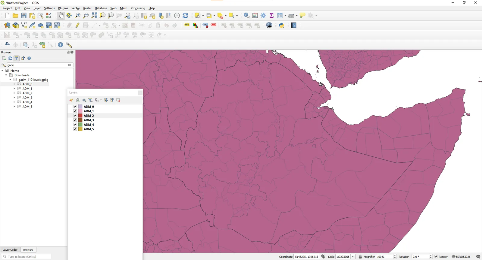
Step 1: Importing an Orthomosaic

Drag your GeoTIFF into the QGIS canvas. That’s it. Layer > Add Layer > Add Raster Layer works too, but drag-and-drop is faster.

QGIS reads the embedded CRS from the GeoTIFF metadata and assigns it automatically. Check the lower-right corner of the status bar — it shows the project CRS. If your orthomosaic lands in the right place on the map, the CRS matched. If it lands in the middle of the ocean or displays as a tiny speck, you have a projection mismatch.

The most common import error: Your photogrammetry software exported in WGS 84 geographic (EPSG:4326), but your project CRS is set to a projected system like UTM. Or vice versa. QGIS will reproject on-the-fly, but that costs rendering performance. For large drone orthomosaics, you want the layer CRS and project CRS to match.

To check a layer’s CRS: right-click the layer > Properties > Information tab. The CRS is listed under “Information from provider.” If it’s wrong — maybe the processing software embedded the wrong EPSG code — don’t reproject the raster. Use Processing > Toolbox > GDAL > Raster projections > Assign Projection to fix the metadata without touching the pixel data. Reprojecting a 2 GB raster takes time and introduces resampling artifacts. Assigning corrects the label without altering values.

Step 2: Build Pyramids Before You Do Anything Else

Drone orthomosaics are big. A 500-acre site at 2 cm/pixel produces a raster with tens of thousands of rows and columns. Panning and zooming without pyramids is like streaming 4K video on dialup.

Right-click your raster layer > Properties > Pyramids tab. Select all resolution levels. Set the resampling method to “Average” for orthomosaics (preserves color fidelity) or “Nearest Neighbour” for classified rasters. Click “Build Pyramids.” QGIS creates lower-resolution overviews stored alongside your file as a .ovr sidecar. File size increases roughly 30-40 percent, but rendering becomes instant.

This is non-negotiable for any raster over 500 MB. Build pyramids first. Do your analysis second.

Alternatively, from the menu: Raster > Miscellaneous > Build Overviews (Pyramids). Same result, different path.

Step 3: CRS Setup and Reprojection

Every drone deliverable carries a coordinate reference system. Your orthomosaic, DEM, and point cloud all have one embedded. The question is whether they match each other — and whether they match the project your client expects.

Practical CRS rules for drone data:

• Most photogrammetry software exports in WGS 84 UTM. Pix4D, Metashape, and WebODM all default to a UTM zone derived from your flight location. This is usually correct.
• State Plane coordinates are common in U.S. survey work. If your client’s CAD file is in State Plane, you’ll need to reproject. Processing > Toolbox > GDAL > Warp (Reproject) handles this for rasters. Right-click > Export > Save Features As handles vectors.
• Vertical datums matter. Your DEM might be in ellipsoidal heights (WGS 84 ellipsoid) while your client expects orthometric heights (NAVD88). QGIS doesn’t handle vertical datum transformations natively — you’ll need a geoid model applied during processing, not in QGIS. Get this right before export, not after.

To put it plainly: match your project CRS to the delivery CRS your client expects. Do the transformation once, correctly, rather than relying on on-the-fly reprojection for every zoom and pan.

Step 4: Measurement and Analysis Tools

Once the orthomosaic is loaded and rendering cleanly, QGIS gives you a full measurement toolkit.

Measure Tool (Sketching Toolbar). Click the ruler icon or press Ctrl+Shift+M. Measure distances, areas, and angles directly on the orthomosaic. The measurement uses the project CRS, so make sure it’s a projected system — measuring distances in geographic degrees is meaningless for field work.

Raster Value Identification. Click the “Identify Features” tool (Ctrl+Shift+I), then click any pixel on your orthomosaic. QGIS reports the band values — useful for checking NDVI layers, thermal data, or verifying that a DEM pixel reads the elevation you expect.

Raster Calculator. Raster > Raster Calculator opens a full band math engine. Compute NDVI from a multispectral orthomosaic: (NIR - Red) / (NIR + Red). Generate slope from a DEM. Difference two DEMs to calculate cut/fill volumes. The syntax is straightforward — select layers and bands from the list, type the formula, set the output extent and CRS.

Step 5: Contour Generation from a DEM

This is the deliverable clients ask for most often after the orthomosaic itself: contour lines from your drone-derived DEM.

Menu path: Raster > Extraction > Contour.

Settings that matter:

• Input layer: Your DEM raster (not the orthomosaic — the elevation model).
• Band number: Band 1. DEMs are single-band.
• Interval between contour lines: This depends on the project. 1-foot contours for construction grading. 2-foot for site plans. 5-foot or 10-foot for large-area topographic maps. The interval is in the vertical units of your DEM — if it’s in meters, “1” means 1-meter contours.
• Attribute name: Leave as “ELEV” — this stores the elevation value on each contour line for labeling.

Click Run. QGIS generates a vector layer of contour lines. The result will look jagged on high-resolution DEMs because the algorithm follows every pixel boundary. To smooth them: Vector > Geometry Tools > Smooth Geometry. A smoothing iterations value of 3 with an offset of 0.25 produces clean, cartographic-quality contours without shifting them off-location.

Export formats: Right-click the contour layer > Export > Save Features As. Choose DXF for AutoCAD delivery, Shapefile for GIS interoperability, or GeoPackage if you’re staying in QGIS.

Step 6: Point Cloud Visualization

QGIS has supported native LAS and LAZ point cloud rendering since version 3.18. No plugins required — just drag a .las or .laz file into the canvas.

On first load, QGIS builds an index using the PDAL library. This takes a minute for large files (100M+ points) and creates a companion index directory next to your source file. After indexing, the point cloud renders in both the 2D map view and the 3D Map View (View > 3D Map View).

Rendering options: Right-click the point cloud layer > Properties > Symbology. Choose from:

• Attribute by Ramp: Color points by elevation, intensity, return number, or classification. Elevation coloring on a drone-derived point cloud gives you an instant visual of terrain variation.
• Classification: If your point cloud has classification codes (ground, vegetation, building), this renderer displays each class in a distinct color. Most photogrammetry-derived point clouds are unclassified — you’ll need to classify them in CloudCompare or PDAL before importing.
• RGB: If your point cloud carries color data from the drone imagery, this renders true-color points. Dense photogrammetric point clouds almost always have RGB.

Elevation Profile Tool. Click View > Elevation Profile (or Ctrl+Shift+E in some builds). Draw a line across the map and QGIS extracts a cross-section profile from your point cloud. This is how you check a stockpile height, verify a drainage grade, or show a client a terrain cross-section — without leaving QGIS.

Step 7: Point Cloud Processing with PDAL Tools

Starting with QGIS 3.32, the PDAL processing tools are built into the Processing Toolbox — no plugin installation needed. Open Processing > Toolbox and search “point cloud.”

Key algorithms for drone data:

• Clip: Trim a point cloud to your site boundary. Feed it a polygon layer and it cuts the cloud to match.
• Merge: Combine multiple flight point clouds into a single dataset.
• Export to Raster: Convert point cloud elevation data to a raster DEM or DSM. Set the resolution to match your ground sample distance.
• Density: Calculate point density per cell — useful for identifying gaps in your photogrammetric reconstruction.
• Filter: Remove points by classification, return number, or elevation range. Strip vegetation returns to isolate bare earth.

These are multi-threaded. On a modern workstation, clipping 50 million points to a site polygon takes seconds, not minutes.

For advanced filtering and classification workflows — ground classification, noise removal, statistical outlier filtering — PDAL’s command-line tools or CloudCompare remain more capable than what’s in the QGIS toolbox. But for standard drone data tasks, the built-in tools handle 90 percent of what you need without leaving QGIS.

Step 8: Exporting Deliverables

Clients don’t use QGIS. They use AutoCAD, ArcGIS, Google Earth, or a web viewer. Your job is to export in the format they need.

Raster exports (orthomosaic, DEM): Right-click > Export > Save As. Choose GeoTIFF for maximum compatibility. Set the CRS to the client’s required projection. Enable LZW compression — it typically reduces file size by 40-60 percent with no quality loss for continuous-tone imagery. For DEMs, use DEFLATE compression to preserve exact elevation values.

Vector exports (contours, boundary polygons, annotations): Right-click > Export > Save Features As. Choose DXF for CAD delivery — this is what your civil engineer expects. Choose Shapefile for legacy GIS systems. Choose GeoPackage for modern GIS workflows — it’s a single file, supports multiple layers, and doesn’t have the attribute name length limitations that Shapefiles carry.

KML/KMZ for Google Earth. Right-click > Export > Save Features As > KML. For raster overlays in Google Earth, use Raster > Conversion > Translate to convert your GeoTIFF to a format Google Earth handles, or export as KMZ tiles using the QTiles plugin.

Print layouts for PDF reports. Project > New Print Layout. Add your orthomosaic as the map element, overlay contours, add a scale bar, north arrow, title block, and legend. Export as PDF at 300 DPI. This is how you deliver a professional map sheet without touching Adobe Illustrator.

Step 9: Field Review with QField

You’ve built your map in QGIS. Now the project manager needs to see it on-site — on a tablet, in the field, with the orthomosaic and contours overlaid on their GPS location.

QField is the answer. It’s the official mobile companion to QGIS — free, open-source, available on Android and iOS.

The workflow:

1. Install the QFieldSync plugin in QGIS. Plugins > Manage and Install Plugins > search “QFieldSync” > Install.
2. Package your project. In QGIS, go to Plugins > QFieldSync > Package for QField. This exports your project, layers, and data into a portable folder optimized for mobile rendering. Large rasters get downsampled automatically — you won’t be loading a 2 GB orthomosaic on a tablet.
3. Transfer to the device. Copy the packaged folder to the tablet via USB, cloud storage, or QFieldCloud for automatic sync.
4. Open in QField. The project loads with all your layers, symbology, and labeling intact. Pan, zoom, and identify features on the orthomosaic. Add field observations as point features with photos and notes.
5. Sync back. Transfer updated data back to QGIS. Any features added in the field appear in your desktop project.

QField supports external GNSS receivers via Bluetooth — connect an Emlid, Trimble, or Bad Elf receiver and your field observations inherit sub-meter or centimeter positioning. That turns QField from a map viewer into a field data collection tool that feeds directly back into your QGIS project.

Common Mistakes and How to Avoid Them

Loading a massive raster without pyramids. QGIS will render it. Eventually. Build overviews first.

Wrong CRS on import. Your orthomosaic appears as a speck or lands in the wrong hemisphere. Check the layer CRS in Properties > Information. Assign the correct projection — don’t reproject unless you actually need to change coordinate systems.

Measuring in geographic coordinates. The Sketching Toolbar measure tool uses the project CRS. If your project is in EPSG:4326 (degrees), distance measurements are in degrees — useless for field work. Switch to a projected CRS before measuring.

Contour artifacts from noisy DEMs. Photogrammetric DEMs have noise — especially in vegetated areas. Run a Gaussian filter (Raster > Analysis > Roughness, or use the SAGA Gaussian Filter in the Processing Toolbox) on the DEM before generating contours. This produces smoother, more cartographically accurate lines.

Point cloud rendering performance. A 200-million-point cloud will choke QGIS on most hardware. Use the PDAL clip tool to trim to your area of interest, or reduce point density before loading. Set the point cloud rendering to “Maximum screen space error” of 3-5 pixels in the layer properties — this thins the display at zoomed-out scales without altering the data.

Bottom Line

QGIS handles the full drone data workflow — orthomosaic display, DEM analysis, contour generation, point cloud visualization, deliverable export, and field review via QField. All of it without a license fee. The 3.44 LTR is stable, the PDAL point cloud tools are mature, and the QField mobile integration closes the office-to-field loop.

The learning curve is real. QGIS doesn’t hold your hand the way commercial software does. But once you’ve built your first project template — CRS configured, pyramids built, print layout saved, QField package ready — every subsequent project is drag-and-drop. The time investment pays for itself on project two.

For practitioners already using commercial GIS, QGIS is worth having in the stack as a second tool — especially for clients who need deliverables but don’t have their own GIS licenses. Hand them a QField project instead of a 2 GB TIFF and a prayer.